Example 1: 1D Diffusion Equation

Problem description and serial Fortran program

We consider the one-dimensional (1D) diffusion equation for $f\left(x,t\right)$ in a periodic domain $x\in \left[-1,1\right],$

$\frac{\partial f}{\partial t}=D\frac{{\partial }^{2}f}{\partial x^2}$,

where $D$ is the diffusion coefficient. Finite differentiations of derivatives yield the expression,

$\frac{f_i^{n+1}-f_i^n}{\mathrm{\Delta t}}=D\frac{f_{i+1}^n-2f_i^n+f_{i-1}^n}{{\left(\mathrm{\Delta x}\right)}^2}$.

$\mathrm{\Delta t}$ is the time step and $\mathrm{\Delta x}$ is the grid spacing. Space and time are discretized by $t_n=n\mathrm{\Delta t}+t_0,x_i=i\mathrm{\Delta x}+x_0$ , where $t_0$ and $x_0$ are the origins (nothing depends on them). $f_i^n$ denotes the value of $f$ on the grid $i$ at the time step $n$. By solving the equation for $f_i^{n+1}$ , we obtain

$f_i^{n+1}=f_i^n+\frac{D\mathrm{\Delta t}}{{\left(\mathrm{\Delta x}\right)}^2}\left(f_{i+1}^n,-,2,f_i^n,+,f_{i-1}^n\right)$.

The expression means that we can calculate $f$ at the next time step $n+1$ from $f$ at the current time step $n$. This finite difference solution of the 1D diffusion equation is coded by Fortran 90 as follows. (If the source code is not shown, please refer this sample code.)

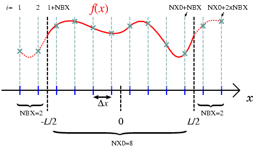
Grid arrangement in the program is shown in Fig. 1. The domain size $L$ is given by LENGTH, and the origin of space coordinate is chosen to be $x_0=-L/2-\mathrm{\Delta x}/2$. The number of grids in the domain and outside the domain are NX0 and NBX, respectively, then the total number of grids becomes nx=NX0+2*NBX. The grids outside the domain are used to calculate the value on the boundary grids. To evaluate the value on the boundary grid (1+NBX), two neighboring grids data (NBX and 2+NBX) are required. In this case, NBX=1 is sufficient. Figure 1 shows more general case in which more grids outside the domain are necessary for higher order finite differentiations. In the grid arrangement shown here, periodic boundary condition is imposed by identifying the data on grids (1:NBX) [(NX0+NBX+1:NX0+NBX+NBX)] with those on grids (NX0+1:NX0+NBX) [(NBX+1:NBX+NBX)].

This program also evaluates the total mass,

$F={\int }_{-L/2}^{L/2}f\text{d}x$,

which conserves during time evolution for the periodic boundary case. Conservation of $F$ is one of a measure of correctness of the numerical solution. The following is a standard output of the program,

	    ./diffuse_serial < diffuse.param.in
time =       0.0000, total =       1.0000, difference =       0.0000 [%]
time =       0.1221, total =       1.0000, difference =      -0.0000 [%]
time =       0.2441, total =       1.0000, difference =       0.0000 [%]
time =       0.3662, total =       1.0000, difference =      -0.0000 [%]
time =       0.4883, total =       1.0000, difference =      -0.0000 [%]
time =       0.6104, total =       1.0000, difference =      -0.0001 [%]
	  

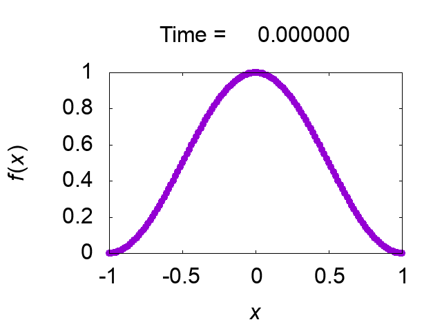
"difference [%]" shows the difference of the total mass from the initial value. The solution looks very good! Figure 2 shows time evolution of the solution.

Parallelization

Parallelization is to distribute uncorrelated tasks to different processors, and to perform those tasks by multiple processors at the same time. Ideal parallelization can reduce elapse time by 1/(number of processors) although ideal means practically impossible (there should be data communications among processors, unbalance of task distribution, unparallelizable tasks, ans so on). In the problem considered here, procedures to calculate $f$ is parallelizable because only values of $f$'s on neighboring grids are necessary. We are going to distribute $f$ to some (or many) processors. Let $N_{\text{p}}$ the number of processors and $N_x$ the number of grids in the domain. $I_{\text{p}}$-th processor ( $I_{\text{p}}=0,\cdots ,N_{\text{p}}-1$ ) is responsible for $N_{\text{min}}$ to $N_{max}$ grids such that

$\begin{array}{ccc}{N}_{\text{min}}& =& \text{int}\left(\frac{N_x}{N_{\text{p}}}\right)I_{\text{p}}+1\\ N_{\text{max}}& =& \text{max}\left(\text{int}\left(\frac{N_x}{N_{\text{p}}}\right)\left(I_{\text{p}}+1\right),N_x\right)\end{array}$,

where $\text{max}\left(a,b\right)$ is a function which returns larger $a$ or $b$, and $\text{int}\left(a\right)$ gives round up of $a$. (Note that, in this division method, the work load may not be even if $N_{\text{p}}$ is large.) The following figure shows a schematic drawing how data are distributed.

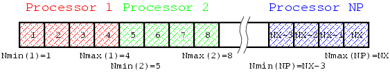
To calculate $f_i^{n+1}$, it is necessary to have neighboring data $f_{i+1}^n$ and $f_{i-1}^n$. However, each processor does not have data required to evaluate the value of the edge grids. For example, suppose $N_x=12$ and $N_{\text{p}}=3$, then, the first to the forth grids are assigned to the first processor, and the fifth grid data is missing to calculate $f$ on the fourth grid. If the periodic boundary condition is considered, processor 1 also need the twelveth grid data which is regarded as equivalent to the zeroth grid. Processor 2 needs the fourth and ninth grids data at each time step, and processor 3 needs the first(=thirteenth) and eighth grids data.

These data transfers among processors are implemented by the help of the MPI library. The following is a possible modification to parallelize by the MPI library. (If the source code is not shown, please refer this sample code.)

Let us see what have been changed in the MPI source code. First of all, we must loudly proclaim that we are in a "parallel world". This is done by use mpi statement in line 11. The MPI module enables us to access the MPI subroutines and predefined parameters. A parallelized part of the MPI source code should be surrounded by the subroutines mpi_init and mpi_finalize. In between those statements, we can use multiple processors. After moving into the parallel world, what each process has to do next is to know who it is (the processor rank) [mpi_comm_rank] and the total number of processors [mpi_comm_size]. In lines from 59 to 66, ranges of grids for which each processor is responsible are determined. Using these ranges, tasks to calculate $f$ are distributed on the processors. As explained earlier, each processor needs to communicate neighboring processors to exchanged neighboring grid data. These communications are performed by subroutine mpi_send and mpi_recv. The calls of the subroutine mpi_gatherv just collect distributed data to one processor for data output. On the other hand, one processor having data sends that data to all other processors by the subroutine mpi_bcast (broadcast). The standard input data are read by only one processor and are broadcasted to other processors.

Communications

Point-to-Point Communications

There are four blocks of data transfers by mpi_send/mpi_recv. Two for the boundary condition, and two for the shift communications that each processor sends/receives edge data. Before calling those MPI subroutines, we define p_send/p_recv which direct each processor the destination/source processors to/from which processor sends/receives data. In the first block (180-200), Processor 0 sends f(NBX+1:NBX+NBX) and processor nps-1 receives it in f(NX0+NBX+1:NX0+NBX+NBX). Thus p_send of processor 0 is nps-1, and p_recv of processor nps-1 is 0. Other processors do nothing in this block. In this case, the destination/source processor rank is defined to be "mpi_proc_null". Mpi_send/mpi_recv in which the destination/source processor is mpi_proc_null return immediately and do nothing.

Collective Communications

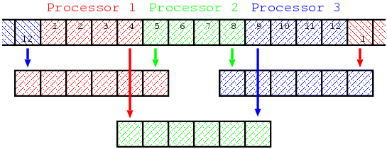
Mpi_gatherv collects data to one processor, and mpi_bcast broadcasts data to all processors. Those subroutines perform data communications collectively among processors defined by the communicator (mpi_comm_world) [usually all processors.]

Data Input/Output (I/O)

In the MPI programs, data I/O of the distributed data must be carefully designed. Although it is easier and safer to force a single processor to do data I/O, such a method may require extra communications or may be just impossible in the first place when handling huge data because a single memory can not accomodate that huge data. On the other hand, in the case where each processor does I/O using separate files, the number of files increases with the number of processors, and file handling will be a mess. It is also possible to do I/O with multi processors in a single file (parallel I/O). In the sample program, the method where one processor does data I/O is taken for simplicity.

Note for Fortran Users

In the C language version of the MPI library, MPI subroutine's return value gives an error code. However, Fortran subroutines do not return a value. An error code is given by the last argument in Fortran version MPI subroutines. This is why all Fortran MPI subroutines take one more integer argument compared to the C version subroutines for an error code. Usually this error code is not referred in programs because the program immediately crashes if an error occurs.

Communicator

Mpi_comm_world is the communicator which encompasses a group of processors that may communicate each other. The communicator is a tag in simple sense. Don't worry about this. Just use this as a communicator.

Deadlock

You may consider that it is possible to combine the communications for the periodic boundary (lines 188-200 and 202-214) with the shift communications (lines 216-227 and 229-240) by defining p_send/p_recv properly. This can be done by setting p_recv=nps-1/p_send=0 in line 222-223, p_recv=0/p_send=nps-1 in line 235-236 to absorb lines 188-214 into lines 216-240. This program, however, may not work in some systems. Mpi_send is the blocking communication subroutine which blocks the following operations until the subroutine successfully copies the data to be sent into the system buffer and returns. Top panel of Figure 5 shows data flow of send/recv communications on the system which has enough buffer. The send/recv communications succeed as shown in the figure. If the system which does not have enough system buffer (see bottom panel of Figure 5), mpi_send called by some processors do not return and other processors should wait for those processes to return. The program does not proceed any further. This situation in which all processors are waiting is called "deadlock."

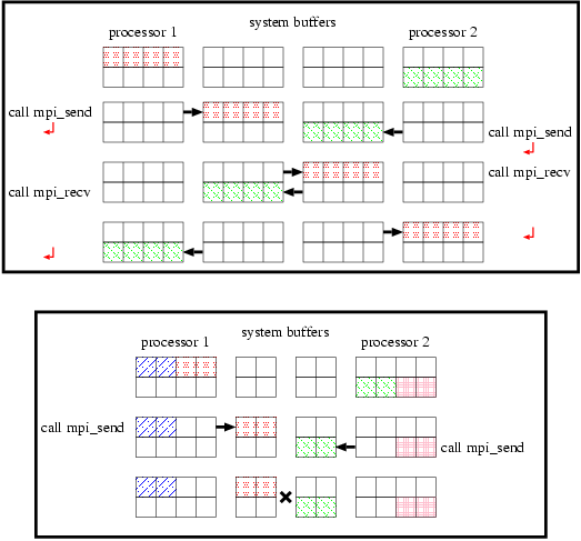
If we change the order of calling mpi_send and mpi_recv, the situation becomes worse. The program obviously deadlocks in all systems (not depend on the size of a system buffer) after all processors call mpi_recv because mpi_recv is also blocking, and returns after receiving the corresponding data.

There are several ways to avoid deadlock. If one processor call mpi_send and the corresponding processor call mpi_recv, this communication succeeds even if the system buffer is not large enough to store all the data to be sent (Figure 6).

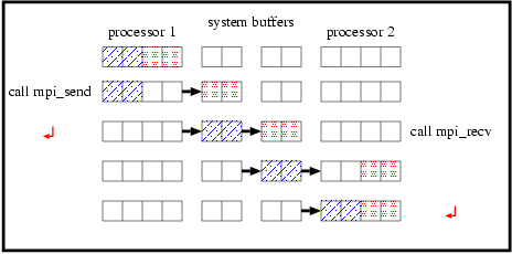
Thus, the source code should be modified for even/odd rank processors to call mpi_send/mpi_recv first. There is a subroutine mpi_sendrecv which automatically do this.

Another way to avoid deadlock is to use the non-blocking communication subroutines. Mpi_isend and mpi_irecv are the non-blocking subroutines which immediately return. The reason for using blocking communication subroutines is to assure correctness of the data to be communicated. This means, in turn, non-blocking subroutines do not avoid illegal access to the data. This can be easily seen by the behavior of mpi_irecv. If we call mpi_irecv(recvbuf,...) and access recvbuf right after the subroutine call,

	      call mpi_irecv(recvbuf,....)
tmp=recvbuf*recvbuf
	    

recvbuf may not have a correct value since it is not guaranteed that mpi_irecv has already received recvbuf. A similar thing can be occurred to mpi_isend. You may overwrite the data to be sent unexpectedly if you access that data immediately after calling mpi_isend. To wait until mpi_irecv/mpi_isend receives/sends data, we can use subroutine mpi_wait. Alteration to use the non-blocking communication subroutines can be as follows,

	      call mpi_isend(sendbuf,...,ireq1,...)
call mpi_irecv(recvbuf,...,ireq2,...)
call mpi_wait(ireq1,...)
call mpi_wait(ireq2,...)
	    

	      total0=sum(f(npmin(pid):npmax(pid)))*dx
call mpi_reduce(total0,total,1,mpirealtype,mpi_sum,rootproc,mpi_comm_world,ierr)
	    

Derivative Type

The most important issue for MPI programming is to reduce time for data communications. Since calling an MPI communication subroutine takes time, it can be efficient to decrease the number of MPI subroutine calls. In the example source code, there are three mpi_bcast calls in lines 55-57. If we can combine them into one mpi_bcast call, it may reduce communication time. (In reality, this modification is not efficient at all. This is just an example to show what a derivative type is.)

The MPI library provides a framework to construct a group of data to be communicated. Users can create a data type of a group of data called a derivative type, and use it as a general MPI data type. To construct a derivative type, we have to define elements of the group. Data types, positions, and sizes of the data are necessary informations.

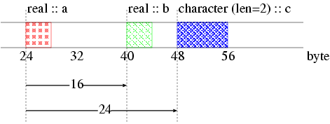
In Figure 7, we show an example of a group of data. The group includes two reals (a and b) and one character (c) of length 2. Positions of data are given by displacements relative to the address of the first data (a). Then, the positions of a, b and c are 0, 16, 24, respectively. The following subroutine defines a derivative type (newtype) can be used in the example source code,

	      subroutine inputtype(int1,int2,int3,newtype)

  use mpi

  implicit none

  integer, intent(in) :: int1,int2,int3
  integer, intent(out) :: newtype
  integer, parameter :: count=3
  integer :: i
  integer (kind=mpi_address_kind) :: addr_start
  integer :: blen(count)
  integer (kind=mpi_address_kind) :: disp(count)
  integer :: tlst(count)

  integer :: ierr

  blen=(/ 1,1,1 /)

  tlst=(/ mpi_integer,mpi_integer,mpi_integer /)

  call mpi_get_address(int1,disp(1),ierr)
  call mpi_get_address(int2,disp(2),ierr)
  call mpi_get_address(int3,disp(3),ierr)
  addr_start=disp(1)
  do i=1,count
     disp(i)=disp(i)-addr_start
  end do

  call mpi_type_create_struct(count,blen,disp,tlst,newtype,ierr)
  call mpi_type_commit(newtype,ierr)

  return

end subroutine inputtype
	    

The group of data has three elements (int1=NX0, int2=NT, int3=NOUT). A size, a data type, and a position of each element are stored in blen, tlst, and disp. Mpi_get_address is used to determine a byte address of each data. The defined group of data is constructed by mpi_type_create_struct. A new data type (newtype) becomes available after committed by mpi_type_commit. Finally, we can broadcast the bunch of data (NX0, NT, NOUT) by calling only one mpi_bcast using the new data type like,

	      call mpi_bcast(nx0,1,intype,rootproc,mpi_comm_world,ierr)
	    

This operation broadcasts (NX0, NT, DATAFILE) altogether, not just NX0.

Set of source codes and adjuncts

From the Subversion Repository, follow public→tutorials→diffuse, and download the source codes.

	      make
	    

	      make MPI=16