Turbulence and Transport
Turbulence (a rough sketch)
Turbulence is a ubiquitous phenomenon. Whenever fluids are set into motion, turbulence tends to develop. As we experience everyday, milk poured into coffee cup shows complex behavior. We stir coffee and milk because we empirically know that turbulence effectively enhances mixing. In the other limit of a spatial scale, we can observe turbulence dominated by the gravitational force in astrophysical objects. Fusion plasma is also a good example of turbulence, in which the electromagnetic forces play important roles. Unfortunately in this case, turbulence makes it extremely difficult to control plasma behavior to confine it into a container.
 |
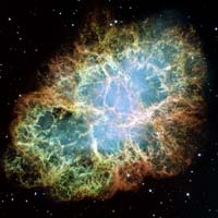
(remnant of supernova explosion) [Image courtesy of HUBBLESITE] |
[Image taken from evl] |
Turbulence is a flow field which is randomly varying in space and time. Though there is no clear definition of turbulence, it has two important properties. One is its sensitive dependence on the initial conditions. Turbulence is, unlike to the laminar flow, unstable, and it changes its pattern drastically because of very slight difference of conditions. Suppose there are two flows which have small differences at some time, those differences grows exponentially in time, and result in thoroughly different flows. It is impossible to reproduce the same flow patterns by controlling turbulence, or to predict behavior of turbulent for a long time. Another important aspect of turbulence is its strong mixing effect. Milk in coffee, pollutants in the atmosphere, temperature in bath, etc. are rapidly diffused by turbulence. Mixing of fuel and oxygen in jet engines enhances the combustion efficiency.
To understand turbulence strongly benefits our human life. After the Reynolds' "discovery" of turbulence, a lot of efforts have been devoted to study turbulence. One most important progress of turbulence theory was made by Russian mathematician A.I. Kolmogorov in 1941. He considered the statistical property hidden in turbulce. For the high Reynolds number developed turbulence, the energy spectrum obeys the law () in the "inertial range" where neither the external force nor the viscous dissipation play roles. This Kolmogorov's similarity law surprisingly fit to observed turbulence. To reveal the universal law hidden in random turbulence motion is a goal.
Simulation of Modified 2D Hasegawa-Wakatani Model
The modified Hasegawa-Wakatani (HW) model describes electrostatic resistive drift wave turbulence in a s tokamak edge plasma, which is written in the form of time evolution of fluctuations of the electrostatic potential () and the density () in a strong equilibrium magnetic field and nonuniform density. The HW model is a generalization of the Hasegawa-Mima (HM) equation including election resistivity parallel to the magnetic field. This parallel electron motion brings about coupling between the vorticity () and the density through the Ohm's law. [In the HM model, the electron resistivity is negligibly small, and electrons obey the Boltzmann relation ().]
"Modification" from the original HW model is attributed to treatment of zonal (poloidally symmetric) components of fluctuations. In a two-dimensional version of the HW model, the resistive coupling between the vorticity and the density does not act on the zonal components. It is therefore necessary to subtract the zonal components from the resistive coupling term.
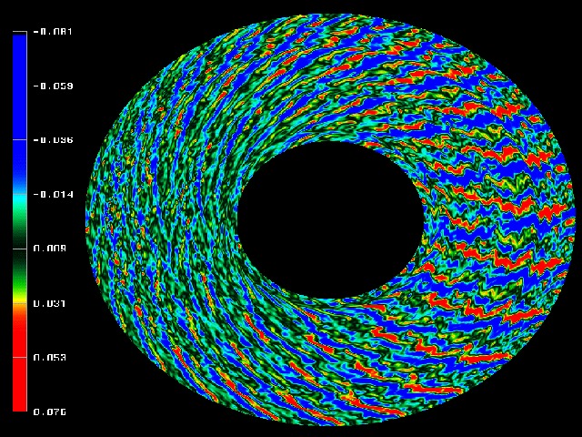
Above animation shows time evolution of , and in a poloidal plane obtained by solving the MHW model numerically. Since the electrostatic potential is nothing but the plasma flow streamfunction, contour plot of shows flow structure. We can observe that zonally elongated (in direction) couter-streaming flows are self-organized by turbulent interaction.
[The term "zonal flow" originally comes from planetary (Earth, Jupiter, etc.) atmospheric flow research.]
Bifurcation in Modified Hasegawa-Wakatani Model
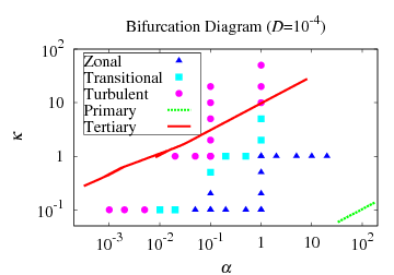
As the zonal flows become too energetic via the feed of energy from the drift wave turbulence, they are subject to instability which breaks up coherent zonal structuring of the flow into turbulent small scale eddies. Therefore, what you observe as a final state may be the state where the zonal flows dominate (as the above figure) or the turbulence dominates depending on parameters of the system. The following figure is a diagram of the final state obtained from the numerical simulations mapped onto the two parameter space spanned by and . (Basically, is the strength of the drive of turbulence, is the resistive dissipation rate.)
[Reprinted with permission from R. Numata, R. Ball and, R. L. Dewar, "Bifurcation in electrostatic resistive drift wave turbulence," Phys. Plasmas 14, 102312. Copyright 2007, AIP Publishing. This article may be downloaded for personal use only. Any other use requires prior permission of the author and the AIP Publishing.]
More strongly the system is driven ( increases) or less resistive the system is ( decreases), more turbulent the system becomes. The green and red lines in the figure denote anlytical prediction of the stability boundaries: beyond the greed [red] line, the drift wave [the zonal flows] become unstable. We see from the figure that the system is coherent rather than turbulent until the zonal flow instability occurs. This phenomenon of upshift of turbulence onset is an analogue of the phenomena known as the "Dimits shift" in a different model (ion-temperature-gradient driven turbulence).
References
-
Bifurcation in electrostatic resistive drift wave turbulence,
R. Numata, R. Ball, R. L. Dewar, Physics of Plasmas 14, 102312 (2007).